Investigate prior

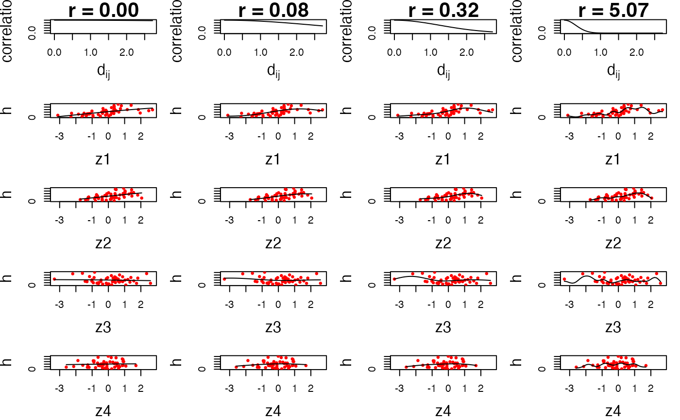
Investigate the impact of the r[m] parameters on the smoothness of the exposure-response function h(z[m]).

Usage

InvestigatePrior(
  y,
  Z,
  X,
  ngrid = 50,
  q.seq = c(2, 1, 1/2, 1/4, 1/8, 1/16),
  r.seq = NULL,
  Drange = NULL,
  verbose = FALSE
)

Arguments

y

a vector of outcome data of length n.

Z

an n-by-M matrix of predictor variables to be included in the h function. Each row represents an observation and each column represents an predictor.

X

an n-by-K matrix of covariate data where each row represents an observation and each column represents a covariate. Should not contain an intercept column.

ngrid

Number of grid points over which to plot the exposure-response function

q.seq

Sequence of values corresponding to different degrees of smoothness in the estimated exposure-response function. A value of q corresponds to fractions of the range of the data over which there is a decay in the correlation cor(h[i],h[j]) between two subjects by 50%.

r.seq

sequence of values at which to fix r for estimating the exposure-response function

Drange

the range of the z_m data over which to apply the values of q.seq. If not specified, will be calculated as the maximum of the ranges of z_1 through z_M.

verbose

TRUE or FALSE: flag indicating whether to print to the screen which exposure variable and q value has been completed

Value

a list containing the predicted values, residuals, and estimated predictor-response function for each degree of smoothness being considered

Details

For guided examples, go to https://jenfb.github.io/bkmr/overview.html

Examples

## First generate dataset
set.seed(111)
dat <- SimData(n = 50, M = 4)
y <- dat$y
Z <- dat$Z
X <- dat$X

priorfits <- InvestigatePrior(y = y, Z = Z, X = X, q.seq = c(2, 1/2, 1/4, 1/16))
PlotPriorFits(y = y, Z = Z, X = X, fits = priorfits)