The package I choose.
Package: bkmr
Research Question
- The cost distribution under different variables.
- The association between Room and board and Tuition for in-state residents (Total cost).
- Try to use Bayesian kernel machine regression to explore unlinear assocition between multivariables and cost.
Original Data
- Data was downloaded from TidyTuesday. The data this week comes from many different sources but originally came from the US Department of Education. Tuition and fees by college/university for 2018-2019, along with school type, degree length, state, in-state vs out-of-state from the Chronicle of Higher Education. Data Source
Data Dictionary
- Here is a data dictionary for what all the column names mean: data dictionary
Load the data into R
Download example data from github and save them in the local site.
if (!require("tidyverse", quietly = TRUE)) {
    install.packages("tidyverse", repos = "http://cran.us.r-project.org")
}
#> ── Attaching core tidyverse packages ──────────────────────── tidyverse 2.0.0 ──
#> ✔ dplyr     1.1.2     ✔ readr     2.1.4
#> ✔ forcats   1.0.0     ✔ stringr   1.5.0
#> ✔ ggplot2   3.4.3     ✔ tibble    3.2.1
#> ✔ lubridate 1.9.2     ✔ tidyr     1.3.0
#> ✔ purrr     1.0.2
#> ── Conflicts ────────────────────────────────────────── tidyverse_conflicts() ──
#> ✖ dplyr::filter() masks stats::filter()
#> ✖ dplyr::lag()    masks stats::lag()
#> ℹ Use the conflicted package (<http://conflicted.r-lib.org/>) to force all conflicts to become errors

if (!require("tidytuesdayR", quietly = TRUE)) {
    install.packages("tidytuesdayR", repos = "http://cran.us.r-project.org")
}

if (!require("here", quietly = TRUE)) {
    install.packages("here", repos = "http://cran.us.r-project.org")
}
#> here() starts at /Users/gsn/Desktop/2023-2024/【JHU】Term-2/【Core】Statistical Programming Workflow/bkmr

if (!require("ggplot2", quietly = TRUE)) {
    install.packages("ggplot2", repos = "http://cran.us.r-project.org")
}

if (!require("purrr", quietly = TRUE)) {
    install.packages("purrr", repos = "http://cran.us.r-project.org")
}
library(here)
library(purrr)

## Test if a directory named data exists locally. If it does not, write an R function that creates it programmatically. Saves the data only once
if (!file.exists(here("data", "tuesdata_tution_cost.csv"))) {

    tuesdata <- tidytuesdayR::tt_load('2020-03-10')
    tuition_cost <- tuesdata$tuition_cost
    tuition_income <- tuesdata$tuition_income


    save_directory <- here("data") # File for saving data, must be created
    if (!dir.exists(save_directory)) {
      dir.create(save_directory, recursive = TRUE)
    }

    # save the files to csv objects ()
    write.csv(tuesdata$tuition_cost, file = here("data", "tuesdata_tuition_cost.csv"))
    write.csv(tuesdata$tuition_income, file = here('data', 'tuesdata_tuition_income.csv'))

}
#> --- Compiling #TidyTuesday Information for 2020-03-10 ----
#> --- There are 5 files available ---
#> --- Starting Download ---
#>
#>  Downloading file 1 of 5: `diversity_school.csv`
#>  Downloading file 2 of 5: `historical_tuition.csv`
#>  Downloading file 3 of 5: `salary_potential.csv`
#>  Downloading file 4 of 5: `tuition_cost.csv`
#>  Downloading file 5 of 5: `tuition_income.csv`
#> --- Download complete ---
## Read in the data locally each time you knit/render
tuition_cost <- read.csv(here("data", "tuesdata_tuition_cost.csv")); tuition_cost$X = NULL
tuition_income <- read.csv(here("data", "tuesdata_tuition_income.csv")); tuition_income$X = NULL
library(tidyverse)
library(stringr)

# 1. Start with tuition cost dataset and drop any rows with NAs.
tuition_cost <- tuition_cost %>%
  drop_na()

# 2. Convert the state names (character strings) to all upper case.
tuition_cost <- tuition_cost %>%
  mutate(state = str_to_upper(state))

# 3. Create new column titled state_code_type that combines the state_code and school type into one column separated by “-”. (e.g. “TX-Private”).
tuition_cost <- tuition_cost %>%
  unite(state_code_type, state_code, type, sep = '-')
# calculate the distribution of room and board of different schooles
tuition_cost_summary <- tuition_cost %>%
  group_by(state_code_type) %>%
  summarise(
    mean_room_and_board = mean(room_and_board),
    sd_room_and_board = sd(room_and_board))

head(tuition_cost_summary)
#> # A tibble: 6 × 3
#>   state_code_type mean_room_and_board sd_room_and_board
#>   <chr>                         <dbl>             <dbl>
#> 1 AK-Private                    6500              1131.
#> 2 AK-Public                    10832.             2070.
#> 3 AL-Private                    8800.             2366.
#> 4 AL-Public                     6994.             2815.
#> 5 AR-Private                    8147.             1670.
#> 6 AR-Public                     7315.             2024.
# calculate the distribution of body mass of penguins
tuition_cost_summary2 <- tuition_cost %>%
  select(-room_and_board) %>%
  group_by(state_code_type, degree_length) %>%
  summarise(
    mean_in = mean(in_state_tuition),
    sd_mass = sd(in_state_tuition))
#> `summarise()` has grouped output by 'state_code_type'. You can override using
#> the `.groups` argument.

head(tuition_cost_summary2)
#> # A tibble: 6 × 4
#> # Groups:   state_code_type [4]
#>   state_code_type degree_length mean_in sd_mass
#>   <chr>           <chr>           <dbl>   <dbl>
#> 1 AK-Private      4 Year         15065    8153.
#> 2 AK-Public       2 Year          4300      NA
#> 3 AK-Public       4 Year          7622.    501.
#> 4 AL-Private      4 Year         18896.   8853.
#> 5 AL-Public       2 Year          5433.   1758.
#> 6 AL-Public       4 Year         10805.    920.
# combine the observed data and summarized result
tuition_cost_combined <- left_join(tuition_cost, tuition_cost_summary, 'state_code_type')
head(tuition_cost_combined)
#>                                   name      state state_code_type degree_length
#> 1         Abilene Christian University      TEXAS      TX-Private        4 Year
#> 2 Abraham Baldwin Agricultural College    GEORGIA       GA-Public        2 Year
#> 3            Academy of Art University CALIFORNIA   CA-For Profit        4 Year
#> 4               Adams State University   COLORADO       CO-Public        4 Year
#> 5                   Adelphi University   NEW YORK      NY-Private        4 Year
#> 6         Adirondack Community College   NEW YORK       NY-Public        2 Year
#>   room_and_board in_state_tuition in_state_total out_of_state_tuition
#> 1          10350            34850          45200                34850
#> 2           8474             4128          12602                12550
#> 3          16648            27810          44458                27810
#> 4           8782             9440          18222                20456
#> 5          16030            38660          54690                38660
#> 6          11660             5375          17035                 9935
#>   out_of_state_total mean_room_and_board sd_room_and_board
#> 1              45200            9228.690          3037.913
#> 2              21024            9383.154          1844.827
#> 3              44458           13824.000          3993.739
#> 4              29238            9853.188          2384.372
#> 5              54690           11868.307          4704.870
#> 6              21595           12582.260          2289.362
tuition_cost_combined %>%
  ggplot(aes(x = room_and_board, y = in_state_total)) +
  geom_point(aes(x = room_and_board, y = in_state_total),  linetype = "solid", color = rainbow(1861), size = 1) +
  labs(title = "Association between the Room and board and total tution in state",
       subtitle = 'Point Chart: Room and board (USD) ~ Total tution (USD)',
       caption = "Data from the Chronicle of Higher Education",
       x = "Room and board in (USD)", y = "Total tution (USD)") +
  facet_wrap(~degree_length, ncol = NULL, scales = "free_y") +
  theme_minimal()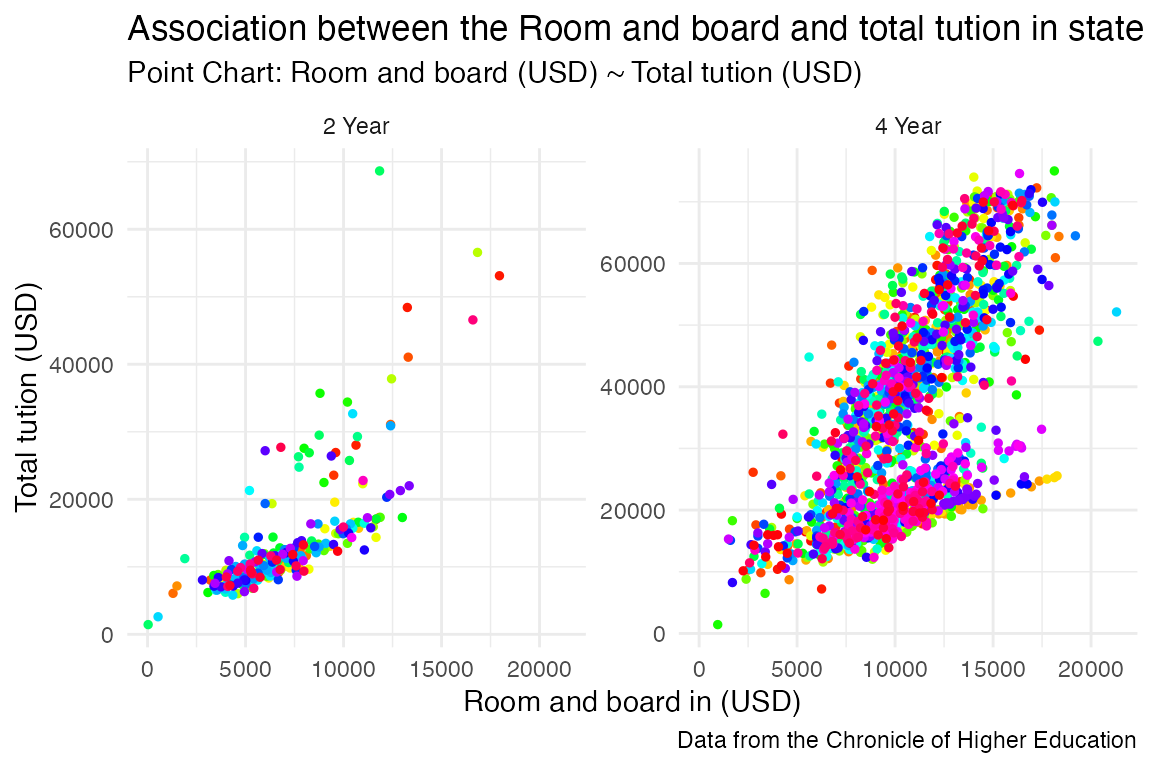
tuition_cost_combined %>%
group_by(state) %>%
filter(room_and_board>10000) %>%
mutate(Mean_diff = out_of_state_total - mean(out_of_state_total)) %>%
ggplot(aes(x = state, y = Mean_diff)) +
geom_histogram(stat = "identity", fill = rainbow(931)) +
labs(title = "The distribution of the total cost out of state difference in each state",
subtitle = 'relative to the mean level at different state',
caption = "Data from the Chronicle of Higher Education",
x = "State", y = "The difference bewteen mean value and observations in each group") +
theme_minimal()+
theme(axis.text.x = element_text(angle = 45, hjust = 1, size=8))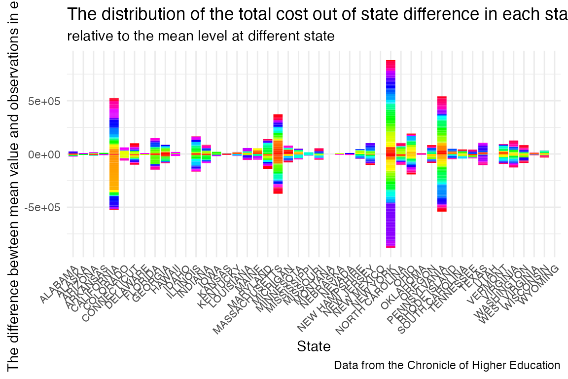 #### BKMR Model Using
reference
#### BKMR Model Using
reference
library(bkmr)
colnames(tuition_cost_combined)
#>  [1] "name"                 "state"                "state_code_type"
#>  [4] "degree_length"        "room_and_board"       "in_state_tuition"
#>  [7] "in_state_total"       "out_of_state_tuition" "out_of_state_total"
#> [10] "mean_room_and_board"  "sd_room_and_board"
data = tuition_cost_combined[, c('room_and_board',
                                 'degree_length',
                                 'mean_room_and_board',
                                 'room_and_board',
                                 'in_state_tuition',
                                 'in_state_total',
                                 'out_of_state_total',
                                 'state')]

data_unique = unique(data[data$out_of_state_total < 20000,])
dat <- SimData(n = dim(data_unique)[1], M = 4) # introduce some nuisance data
Adopt purrr function to facilitate process
## explore linear regression
by_degree <- split(data_unique, data_unique$degree_length)
by_degree |>
  map(.f = ~ lm(out_of_state_total ~ state, data = .x)) |>
  map(.f = coef)
#> $`2 Year`
#>         (Intercept)         stateALASKA        stateARIZONA       stateARKANSAS
#>          12548.5000           4751.5000            881.0714            744.8333
#>     stateCALIFORNIA       stateCOLORADO        stateGEORGIA          stateIDAHO
#>           2599.5000           2048.9000           2105.5000           3759.0000
#>           stateIOWA         stateKANSAS      stateLOUISIANA          stateMAINE
#>           1145.7500          -2841.7222           3875.5000           1621.5000
#>       stateMARYLAND       stateMICHIGAN      stateMINNESOTA    stateMISSISSIPPI
#>           5596.5000           1489.1667          -1316.3000          -2936.3571
#>       stateMISSOURI        stateMONTANA       stateNEBRASKA     stateNEW JERSEY
#>            886.9444           -569.2500          -1423.2500           2556.5000
#>     stateNEW MEXICO       stateNEW YORK   stateNORTH DAKOTA           stateOHIO
#>          -5693.2500           4952.3333            919.8333           3317.0000
#>       stateOKLAHOMA         stateOREGON   statePENNSYLVANIA stateSOUTH CAROLINA
#>           3427.0455           -253.1667           4746.5000           3824.0000
#>          stateTEXAS           stateUTAH     stateWASHINGTON  stateWEST VIRGINIA
#>          -1126.3276            -53.5000            944.0714           7351.5000
#>      stateWISCONSIN        stateWYOMING
#>           3015.7500           1762.9286
#>
#> $`4 Year`
#>         (Intercept)         stateALASKA        stateARIZONA       stateARKANSAS
#>          17392.3333          -2392.3333          -5063.3333            675.0000
#>     stateCALIFORNIA        stateFLORIDA        stateGEORGIA         stateHAWAII
#>          -1894.3333           -411.9333          -1512.3333          -5246.3333
#>          stateIDAHO           stateIOWA         stateKANSAS       stateKENTUCKY
#>          -3677.3333           -207.3333         -15962.3333          -3337.3333
#>      stateLOUISIANA       stateMARYLAND       stateMICHIGAN      stateMINNESOTA
#>          -1136.3333           1607.6667          -6392.3333            374.3333
#>    stateMISSISSIPPI       stateMISSOURI        stateMONTANA       stateNEBRASKA
#>          -1951.4444            424.9167          -6072.3333           -353.5833
#>         stateNEVADA     stateNEW JERSEY     stateNEW MEXICO       stateNEW YORK
#>          -4484.3333            274.3333          -1376.3333          -2790.1410
#> stateNORTH CAROLINA   stateNORTH DAKOTA           stateOHIO       stateOKLAHOMA
#>           -194.7333          -1607.3333          -2355.3333          -2060.8333
#>         stateOREGON   statePENNSYLVANIA stateSOUTH CAROLINA   stateSOUTH DAKOTA
#>           1257.6667          -2942.3333           -279.3333           1733.6667
#>      stateTENNESSEE          stateTEXAS           stateUTAH        stateVERMONT
#>            719.1667          -1987.1111          -4144.3333            891.6667
#>       stateVIRGINIA
#>           1007.6667

## transform data
string_to_integer <- function(column) {
  as.integer(as.factor(column))
}
data_unique[, c(2,8)] <- map_dfc(.x = data_unique[, c(2,8)], .f = tolower)
data_unique[, c(2,8)] <- map(data_unique[, c(2,8)], string_to_integer)
set.seed(208)
data_unique[,c(1:8)] = scale(data_unique[,c(1:8)])

y <- as.matrix(data_unique$out_of_state_total)
Z <- cbind(as.matrix(data_unique[, c(1,2,8)],), dat$Z)
X <- as.matrix(data_unique[, c(3)])
fitkm <- kmbayes(y = y, Z = Z, X = X, iter = 1000, verbose = FALSE, varsel = TRUE)
#> Iteration: 100 (10% completed; 2.49247 secs elapsed)
#> Iteration: 200 (20% completed; 4.85539 secs elapsed)
#> Iteration: 300 (30% completed; 7.19379 secs elapsed)
#> Iteration: 400 (40% completed; 9.61304 secs elapsed)
#> Iteration: 500 (50% completed; 11.9123 secs elapsed)
#> Iteration: 600 (60% completed; 14.22316 secs elapsed)
#> Iteration: 700 (70% completed; 16.64419 secs elapsed)
#> Iteration: 800 (80% completed; 19.08055 secs elapsed)
#> Iteration: 900 (90% completed; 21.48126 secs elapsed)
#> Iteration: 1000 (100% completed; 24.00408 secs elapsed)
ExtractPIPs(fitkm)
#>         variable   PIP
#> 1 room_and_board 1.000
#> 2  degree_length 1.000
#> 3          state 0.680
#> 4             z1 0.168
#> 5             z2 0.178
#> 6             z3 0.262
#> 7             z4 0.004
# A posteriori inclusion probability in a simulated data set (the bigger the better)
#TracePlot(fit = fitkm, par = "r", comp = 1)
#TracePlot(fit = fitkm, par = "sigsq.eps")

pred.resp.univar <- PredictorResponseUnivar(fit = fitkm)
library(ggplot2)
ggplot(pred.resp.univar, aes(z, est, ymin = est - 1.96*se, ymax = est + 1.96*se)) +
    geom_smooth(stat = "identity") +
    facet_wrap(~ variable) +
    labs(title = "The univariate relationship between specific exposure and the total cost",
       subtitle = 'All variables have been standarized to 0~1',
       caption = "Data from the Chronicle of Higher Education",
       x = "Scaled Value", y = "h(z)")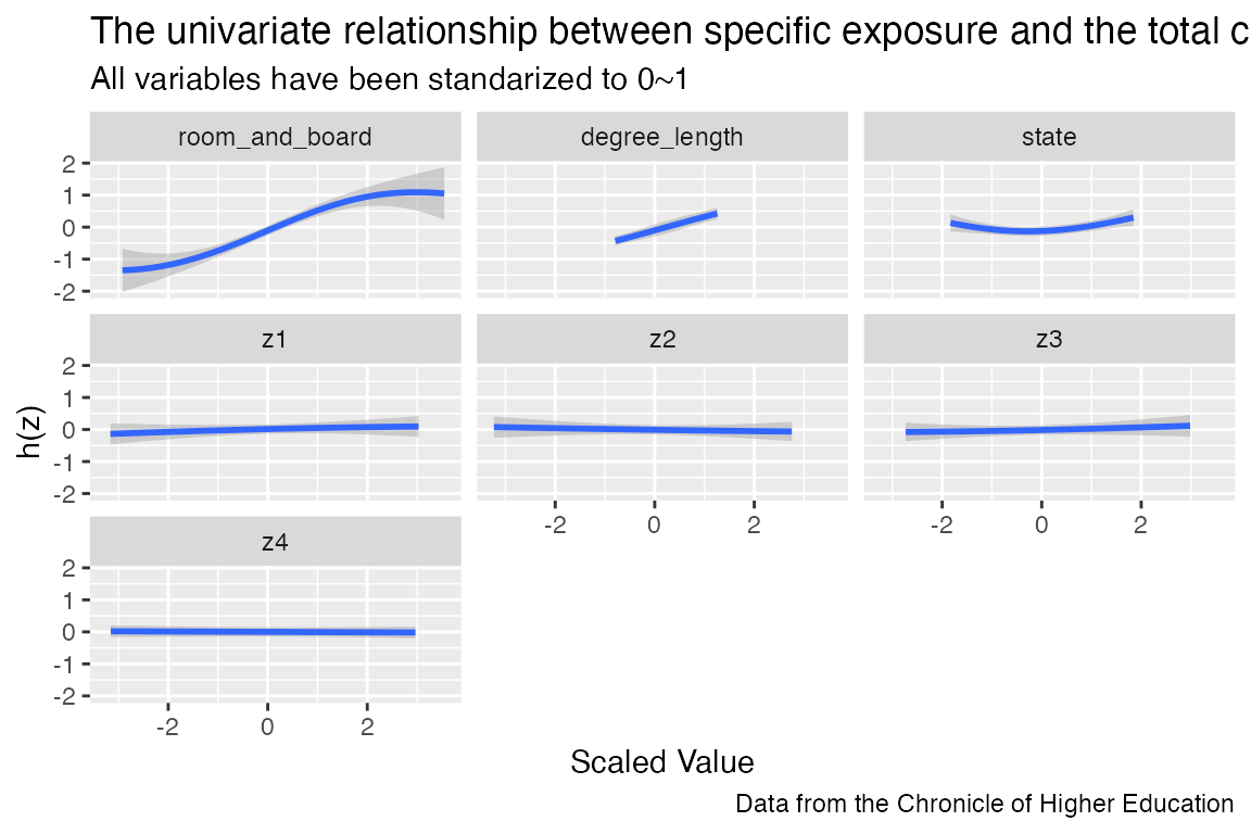
Summary of Analysis
- The school in California, New York, Massachusetts, and Pennsylvania showed the top 4 highest deviation in total cost out of state.
- The total tution in state showed two kinds of linear association with room and board. These two patterns can be detected to explore further.
- Even though we considering nuisance parameter, BKMR could identify the actual effect from room and board cost, degree length and state to total cost with out of state cost smaller than 20000. Also, in the PIP value list, room and board, degeree length and state showed the highest prbability, corrsponding to our expectations.