Trace plot
Usage
TracePlot(
  fit,
  par,
  comp = 1,
  sel = NULL,
  main = "",
  xlab = "iteration",
  ylab = "parameter value",
  ...
)
Arguments
- fit
An object containing the results returned by a the
kmbayesfunction- par
which parameter to plot
- comp
which component of the parameter vector to plot
- sel
logical expression indicating samples to keep; defaults to keeping the second half of all samples
- main
title
- xlab
x axis label
- ylab
y axis label
- ...
other arguments to pass onto the plotting function
Details
For guided examples, go to https://jenfb.github.io/bkmr/overview.html
Examples
## First generate dataset
set.seed(111)
dat <- SimData(n = 50, M = 4)
y <- dat$y
Z <- dat$Z
X <- dat$X

## Fit model with component-wise variable selection
## Using only 100 iterations to make example run quickly
## Typically should use a large number of iterations for inference
set.seed(111)
fitkm <- kmbayes(y = y, Z = Z, X = X, iter = 100, verbose = FALSE, varsel = TRUE)
#> Iteration: 10 (10% completed; 0.00475 secs elapsed)
#> Iteration: 20 (20% completed; 0.01022 secs elapsed)
#> Iteration: 30 (30% completed; 0.01547 secs elapsed)
#> Iteration: 40 (40% completed; 0.02064 secs elapsed)
#> Iteration: 50 (50% completed; 0.02597 secs elapsed)
#> Iteration: 60 (60% completed; 0.03126 secs elapsed)
#> Iteration: 70 (70% completed; 0.03639 secs elapsed)
#> Iteration: 80 (80% completed; 0.04153 secs elapsed)
#> Iteration: 90 (90% completed; 0.04675 secs elapsed)
#> Iteration: 100 (100% completed; 0.05206 secs elapsed)

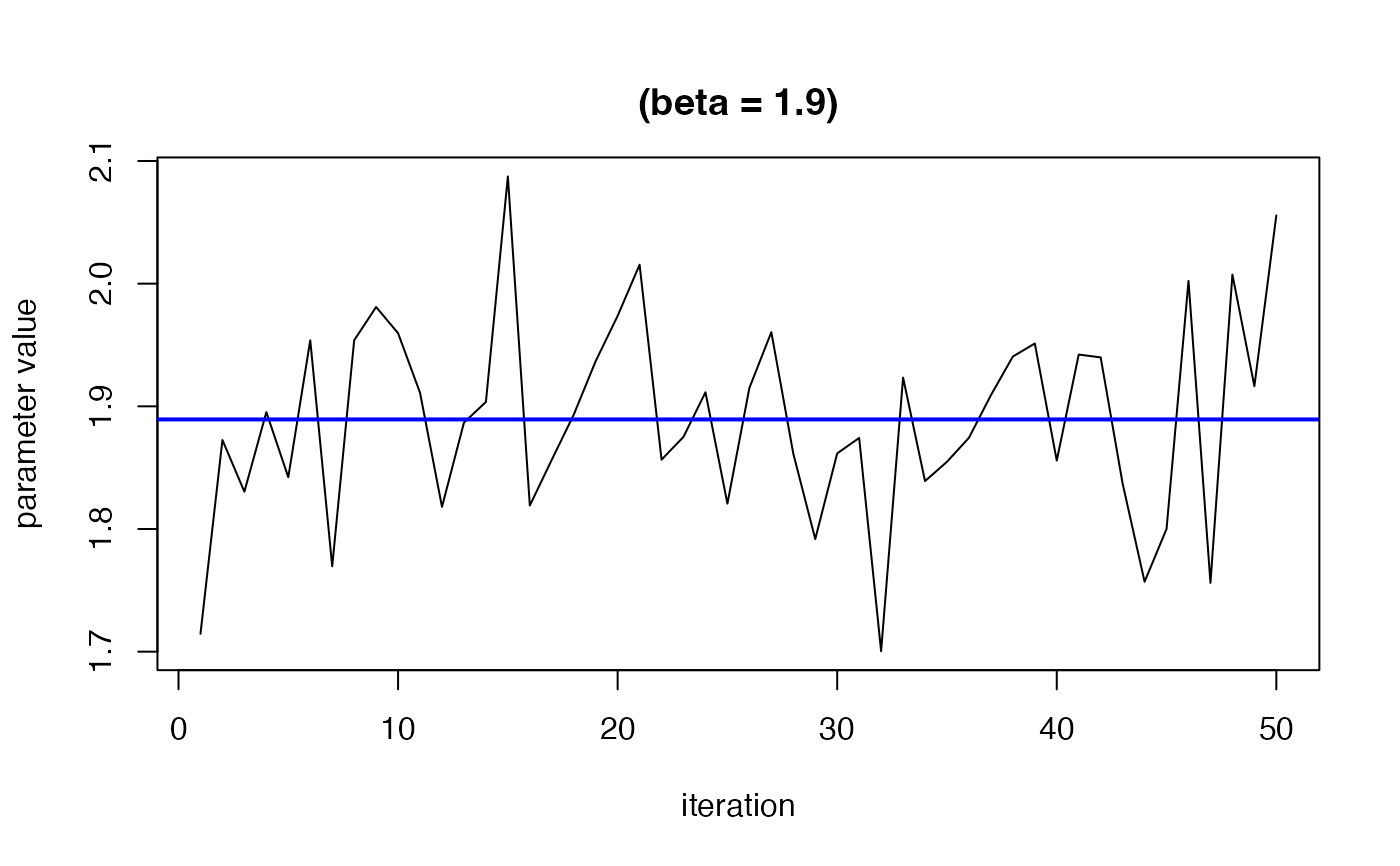
TracePlot(fit = fitkm, par = "beta")

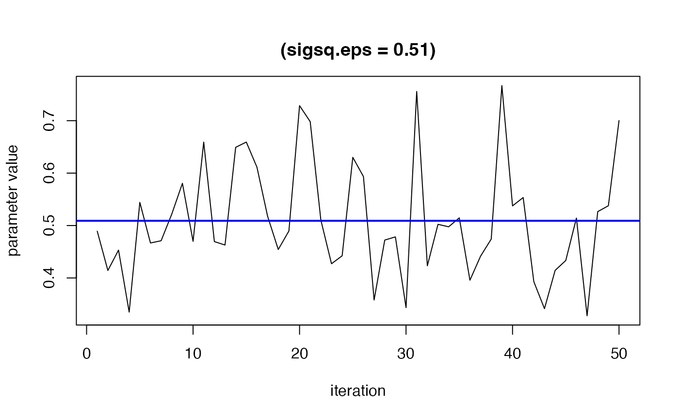
TracePlot(fit = fitkm, par = "sigsq.eps")

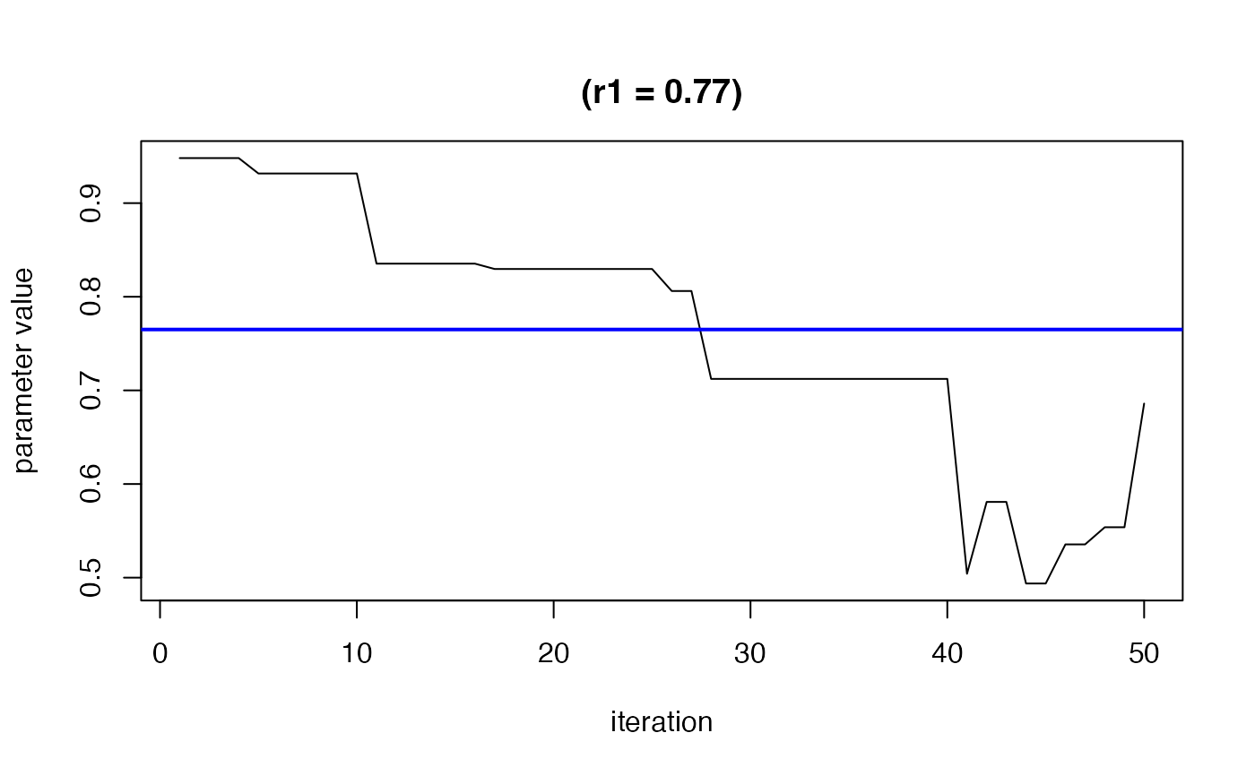
TracePlot(fit = fitkm, par = "r", comp = 1)
